猪瘟病毒栏内和栏间传播:一种通过传播实验估算基本复制比的新方法（上）

　　Within- and between-pen transmission of Classical Swine Fever Virus: a new method to estimate the basic reproduction ratio from transmission experiments - Part 1

　　1

　　作者 Authors:

　　D. KLINKENBERG1, J. DE BREE1, H. LAEVENS2 and M. C. M. DE JONG1

　　1荷兰动物科学与健康研究所，定量兽医传染病学

　　1Institute for animal science and health, quantitative veterinary epidemiology, The Netherlands

　　2比利时根特大学兽医学院兽医流行病学组，生殖、生育和畜群健康系

　　2Department of reproduction, obstetrics and herd health, veterinary epidemiology unit, school of veterinary medicine, Ghent University, Belgium

　　2

　　总结 SUMMARY

　　本文提出了一种从传播实验中估算基本复制比Ro的方法。通过更广泛地使用先前发表的经典猪瘟病毒实验数据，我们得到了比原始论文中使用的鞅方法更小的置信区间。

　　We present a method to estimate basic reproduction ratio Ro from transmission experiments. By using previously published data of experiments with Classical Swine Fever Virus more extensively, we obtained smaller confidence intervals than the martingale method used in the original papers.

　　此外，我们的方法允许同时估算栏内的复制比(ROw)和调整后栏与栏之间的复制比 (R’ob)。对ROw和R 'ob断奶仔猪的估算值分别为100 (95% CI 54-4-186)和7.77(4-68-12. 9)。

　　Moreover, our method allows simultaneous estimation of a reproduction ratio within pens ROw and a modified reproduction ratio between pens R’ob. Resulting estimates of ROw and R’ob weaner pigs were 100 (95% CI 54. 4-186) and 7.77 (4. 68-12. 9), respectively.

　　对于育肥猪来说，这两个数值分别是15. 5 (6. 20-38. 7) 和3. 39 (1. 54-7. 45)。我们认为，由于我们能够获得较小的置信区间，因此本文提出的方法更适合在未来的实验中使用。

　　For slaughter pigs they were 15. 5 (6. 20-38. 7) and 3. 39 (1. 54-7. 45), respectively. We believe, because of the smaller confidence intervals we were able to obtain, that the method presented here is better suited for use in future experiments.

　　3

　　简介 INTRODUCTION

　　猪瘟(CSF)或猪霍乱是一种高度传染性的猪病[1-3]，这种疾病的流行会引起巨大的问题，如动物福利的减少，以及由于出口限制和猪群大规模毁灭而造成的高经济损失[4]，这种疾病是由猪瘟病毒(CS FV)引起的[1-3]。病毒在猪之间的传播可以通过从传播实验中的估算参数来量化，在这些实验中，栏内的一些猪只接种了病毒，并在随后跟踪了传播进程[5]。

　　Classical Swine Fever (CSF) or hog cholera is a highly contagious pig disease [1-3], an epidemic of which can cause huge problems like reduction in animal welfare, and high economic losses as a result of export limitations and mass destruction [4]. The disease is caused by the Classical Swine Fever Virus (CSFV) [1-3]. Transmission of the virus between pigs can be quantified by estimating parameters from transmission experiments, in which a number of pigs within a pen are inoculated with the virus and the transmission process in followed [5].

　　病毒传播的一个重要参数是基本复制比Ro，定义为在无限易感猪群中由一个典型传染性个体引起的继发性感染个体的数量。如果Ro小于1，然后平均每一个有传染性的动物感染的动物少于一个，导致疫情消退。反之，如果Ro大于1，则可能发生重大疫情[6]。

　　An important parameter of virus transmission is the basic reproduction ratio Ro, defined as the number of secondary infected individuals caused by one typical infectious individual in an infinite susceptible population. If Ro is smaller than 1, then on average every infectious animal infects less than one other animal causing the outbreak to wane. If on the other hand Ro is greater than 1, major outbreaks can occur [6].

　　1998年和1999年，Laevens等人用CSFV做了两个传播实验；一个用断奶猪，另一个实验用育肥猪[7,8]。在这两个实验中，有3个相邻的大栏，每个大栏中有15只断奶猪或6只育肥猪。在中间的大栏中一只猪接种了CSFV，每2天采集所有猪的血样检测病毒血症。根据这些测量结果，当一头猪是病毒血症的，就假设这头猪是有传染性的，从而重建了每头猪的感染周期。随后Ro采用鞅估算方法，基于随机SIR模型进行估算[5,9]。

　　In 1998 and 1999 Laevens et al. did two transmission experiments with CSFV; one with weaner pigs and the other with slaughter pigs [7, 8]. In both experiments there were 3 adjacent pens with either 15 weaner pigs or 6 slaughter pigs in each pen. In the middle pen one pig was inoculated with CSFV and every 2 days blood samples of all the pigs were taken to measure viraemia. From these measurements the infectious period of every pig was reconstructed by assuming that a pig is infectious when it is viraemic. Subsequently Ro was estimated using the martingale estimation method, based on the stochastic SIR model [5, 9].

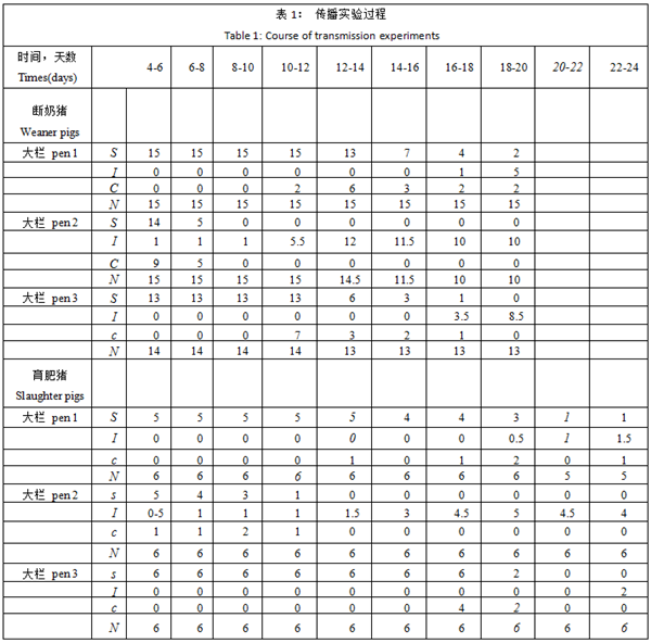
　　注：将病毒传播过程划分为2天时间段，按大栏分层。时间从接种疫苗那天开始。S为区间开始时易感动物的数量；I为受感染动物的数目；C是新病例数，N是动物总数，其中0·5是某一类别2天中只出现1天的动物。

　　Division of the virus transmission process in 2-day time periods, stratified by pen. Time starts at day of inoculation. S is the number of susceptible animals at the start of the interval; I is the number of infectious animals; C is the number of new cases and N is the total number of animals, where 0·5 is an animal present for only 1 of 2 days in a certain category.

　　该模型通过描述易感(S)和传染性(I)动物数量的变化和动物总数(N)来描述病毒在一组动物中的传播。在该模型中，假设易感动物的感染和感染动物的恢复是由速率为βSI/N和α I的泊松过程产生的，其中β和α分别是传播和恢复参数。

　　This model describes transmission of a virus in a group of animals by describing the change in the numbers of susceptible (S) and infectious (I) animals in terms of these numbers and the total number of animals (N). In the model, infection of susceptible animals and recovery of infectious animals are assumed to be generated by a Poisson process with rates βSI/N and αI, where β and α are the transmission and recovery parameter, respectively.

　　Ro是根据实验中最终感染的动物数量来估算的，此时没有易感动物或无传染性动物存在。如果相关，使用最后一个易感动物被感染时剩余的感染期分数之和。Laevens等仅使用中间大栏的数据来估算Ro，因为在其它大栏中，传播并不仅仅是由同一大栏内的传染性动物引起的[7,8]。

　　The Ro is estimated from the number of animals ultimately infected during the experiment, when no susceptible or no infectious animals remain. The sum of the fractions of infectious periods remaining when the last susceptible animal is infected is used if relevant. Laevens et al. [7, 8] used only the data of the middle pen to estimate Ro because in the other pens transmission was not solely caused by infectious animals in the same pen.

　　断奶猪和育肥猪分别得到的估算数据是(s.e. 109, i.e. 95% CI -132-295)和13. 7 (s.e. 13. 7, i.e. 95% CI -13. 2-40. 6) 。这意味着，尽管感染过程发生得非常快，所有动物都被感染了，但估算的Ros并不显著大于1。由于数据的某些方面并没有被用于估算(三个大栏内所有动物的感染时间和感染周期)，因此，尽可能多地利用数据信息，寻找另一种估算方法是值得的。期望这会得到更小的置信空间。

　　The estimates obtained were (s.e. 109, i.e. 95% CI -132-295) and 13. 7 (s.e. 13. 7, i.e. 95% CI —13. 2-40. 6) for weaner and slaughter pigs, respectively. This meant that despite the fact that the infection process took place very quickly and all animals were infected, the estimated Ros were not significantly greater than 1. Since some aspects of the data were not used for the estimation (infection times and infectious periods of all animals known for all three pens), searching for an alternative estimation method would be worthwhile, using as much information from the data as possible. Hopefully this will lead to a smaller confidence interval.

　　为了得到一个较小置信区间的 Ro 估算，我们分别估算了感染性参数β和恢复性参数α，这两个参数用来计算 (Ro =β/α)。 对于β的估算根据已知的感染个案数目(C)、易受感染动物数目(S)及感染动物数目(I)，把感染过程划分为不同的时间间隔。 这些(S, I, C)的集合被用来构造一个概率函数，我们最大化为β得到一个最大概率估算。对α进行估算，以感染周期的长度拟合一个广义线性模型。

　　In an attempt to obtain an Ro estimate with a smaller confidence interval, we did separate estimations of β, the infectivity parameter, and α, the recovery parameter, which are used to calculate Ro (Ro =β/α). For β estimation, the infection process was partitioned into intervals with known numbers of infection cases (C) and susceptible (S) and infectious (I) animals. These sets of (S, I, C) were used to construct a likelihood function, which we maximized to get a maximum likelihood estimator for β. For α estimation, the lengths of the infectious periods were used to fit a generalized linear model.

　　4

　　材料和方法 MATERIALS AND METHODS

　　我们使用了laevens 等人在传播实验中获得的数据(详情请见[7,8])。在两个实验中，有3个相邻的大栏，猪的数量相等: 一个实验中有15头断奶仔猪，另一个实验中有6头育肥猪。在中间的大栏中一只猪接种了CSFV，每2天采集所有猪的血样检测病毒血症。当一头猪是病毒血症的，就假设这头猪是有传染性的，从而重建了每头猪的感染周期。

　　We used the data obtained in the transmission experiments of Laevens et al. (for more detail see [7, 8]). In both experiments there were 3 adjacent pens with equal numbers of pigs: 15 weaner pigs in one experiment and 6 slaughter pigs in the other. One of the pigs in the middle pen was inoculated with CSFV and every 2 days blood samples were taken from all animals, which were tested for viraemia. From these data the infectious period of each pig was reconstructed, assuming that the animal is infectious when it is viraemic.

　　通过假设的潜伏期为6天(已感染但还没有传染性)，我们能够在三个栏中重建整个病毒传播过程[2]。这些重建使我们能够估计参数，使用以下随机SIR模型[6]，包括大栏内和大栏间传播:

　　比率 (S →S -1) = (βwIw/Nw+βbIb/Nb)S (1)

　　比率 (I→I -l) =αI.                     (2)

　　By assuming a latent period of 6 days (infected but not yet infectious) [2], we were able to reconstruct the entire virus transmission process in the three pens. These reconstructions enabled us to estimate the parameters, by using the following stochastic SIR model [6], incorporating both within- and between- pen transmission:

　　rate (S →S -1) = (βwIw/Nw+βbIb/Nb)S (1)

　　rate(I→I -l) =αI.                     (2)

　　在这个模型中，βw是大栏内传播参数，定义为在一个完全易感的群体中，在同一大栏中，每只典型的传染性动物每天新感染的预期数量。同样地，βb是大栏间传播参数，定义为是在完全易感群体中，每个典型传染性动物每天在其他大栏中预期的新感染数量。

　　In this model, βw is the within-pen transmission parameter defined as the expected number of new infections in the same pen per day per typical infectious animal in a fully susceptible population. Likewise, βb is the between-pen transmission parameter defined as the expected number of new infections in other pens per day per typical infectious animal in a fully susceptible population.

　　参数α代表每只感染动物的恢复率。由于有两个传输参数 βw 和βb，我们还区分了大栏内复制比ROw和大栏间复制比ROb。ROw定义为在同一个大栏内一个典型的传染性动物引起的预期继发感染的动物数量。ROb定义为由一种典型的传染性大栏引起的预期继发感染大栏数，考虑到一个大栏被感染，则栏内至少有一头猪被感染。ROw和ROb的估算可以计算如下：

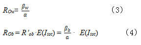
　　The parameter α represents the recovery rate per infectious animal. Because there are two transmission parameters βw and βb，we also make a distinction between a within-pen reproduction ratio ROw and a between-pen reproduction ratio ROb. ROw is defined as the expected number of secondary infected animals caused by one typical infectious animal in the same pen. ROb is defined as the expected number of secondary infected pens caused by one typical infectious pen, considering a pen as infected when at least one pig is infected. Estimates for ROw and ROb can be calculated as follows:

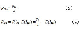
　　在这个等式中，E(Itot)是一个大栏内最终被感染的动物的预估数量。如果ROw是已知的，那么E(Itot)在我们的模型假设条件下容易确定[10],但本文不做进一步探讨。R’ob是指由一种典型的传染性动物引起的继发感染大栏数量的预估数量。R’ob独立于E(Itot)，是本文即将估计的参数。为了便于计数，我们引入了向量 = (βw, βb)，log= (logβw, logβb),  =( ROw, R’ob)，和log = (log ROw,log R’ob)。因为感染和恢复是相互独立的过程，是通过分别估计和计算得出的。

　　In this equation, E(Itot)is the expected number of animals ultimately infected within one pen. E(Itot) can under our model assumptions easily be determined if ROw is known [10], but will not be further discussed in this paper. R’ob is the expected number of secondary infected pens caused by one typical infectious animal. R’ob, being independent of E(Itot), is the parameter that will be estimated in this paper. For notational convenience, we have introduced the vectors  = (βw, βb)，log= (logβw, logβb),  =( ROw, R’ob)，and log = (log ROw,log R’ob). Because infection and recovery are independent processes,  was calculated from separate estimations of  and .

　　为了估计传播参数,，将感染过程分为两天的时间间隔，即两次随后抽样之间的时间间隔。对于每一间隔，间隔开始时易感猪只的数量(S)，具有传染性猪只的数目(I)以及新增病例(C)的数目已确定（表1）。 在每个时间间隔 k 中，易感动物逃脱恒定感染率(βw Iwk /Nwk+βbIbk/Nbk)的概率，按照泊松分布，是e-(βw Iwk /Nwk+βbIbk/Nbk)。 因此，根据二项分布，在同一大栏Ck病例的概率是，Sk易感猪和ik具有传染性的猪只比例(Ik/ Nk) ，jk为其它大栏中具有传染性的猪只比例:

　　用所有时间间隔的概率组成对数似然函数，可以写成:

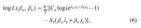
　　在此过程中，log中忽略未计，因为它没有作用。使这个函数最大化，得到了对βw和βb的最大似然估计。

　　In order to estimate transmission parameters, the infection process has been divided into time intervals of two days, the intervals between two subsequent samplings. For each interval, the number of susceptible pigs at the start of the interval (S), the number of infectious pigs (I) and the number of new cases (C) was determined (Table 1). In each time interval k, the probability of a susceptible animal escaping infection from the constant rate (βw Iwk /Nwk+βbIbk/Nbk)  is, according to the Poisson distribution, e-(βw Iwk /Nwk+βbIbk/Nbk).Therefore, the probability of getting Ck cases, with Sk susceptibles and ik as the fraction of infectious pigs (Ik/ Nk) in the same pen and jk as the fraction of infectious pigs in the other pens is, according to the binomial distribution:

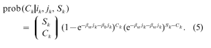
　　The probabilities for all time intervals have been used to make up the log-likelihood function, which may be written as:

　　where log has been omitted because it plays no role. Maximising this function results in maximum likelihood estimators for βw and βb.

　　采用三种方法推导出了βw的置信区间。比较几个特性(如数学背景，实用价值)，然后决定哪些方法应该用于βb和ROw 以及 R’ob的区间估计。第一个方法，我们称之为构建方法，是基于似然比和等价的测试并且构建的置信区间。这里使用的检验是从以下观察得出的：检验一个值(Ho: βw = βo)与另一个值βw (HA: βw =β’< βo )的似然比是每个C的单调递减函数。

　　Three methods were used to derive confidence intervals for βw. After comparing several features (e.g. mathematical background, practical value), a decision was made as to which method should be used for interval estimation of βb，ROw and R’ob .The first method, which we shall refer to as the construction method, is based on the likelihood ratio and on the equivalence of testing and construction of a confidence interval. The test used here is derived from the observation that the likelihood ratio for testing one value of (Ho: βw = βo) against another value of βw (HA: βw =β’< βo ) is a monotonic and decreasing function of each C.

　　它允许我们用C本身的概率函数为C构造一个临界区域，而不需要调用任何近似似然比的概率分布。详情请参阅附录。用这种方法可以构造两个βs (βw or βb)中的一个的置信区间，将另一个作为常数作为其估计。遗憾的是，这种计算几乎是非常耗时的，如何构造参数向量的置信区间或者如何确定Ro的置信区间是不清楚的。第二种方法是Neyman 和 Pearson (参考文献[11])所描述的似然比()检验，它依赖于—21og 的渐近卡方分布，在我们的案例中是1自由度。

　　It allowed us to construct a critical region for the C by using the probability function of C itself，without invoking any approximate probability distribution of the likelihood ratio. For details, see the appendix. With this method confidence intervals can be constructed for one of the two βs (βw or βb) treating the other as a constant as its estimate. Unfortunately, the computation is almost prohibitively time-consuming, and just how to construct a confidence area for the parameter vector or how to determine confidence intervals for Ro is not clear. The second method is the likelihood ratio () test as described by Neyman and Pearson (reference in [11]), which relies on the asymptotic chi-square distribution of —21og with, in our case, 1 degree of freedom.

　　该方法通过求解方程—21og = 3. 84计算95% 置信区间，对于两个βs (βw 或βb)中的一个，将另一个作为常数作为其估计。这是一个比第一个快得多的方法，尽管如此，它在同时置信区间的构造上也存在同样的困难。第三种方法是基于最大似然估计的渐近(多元)正态分布[12]。估计量的假设是由log估计值 (而不是)， 同时也是一个ML-估计值，是渐近正态分布因为非现实(负的)的βw 和 βb不能发生。结果如下协方差矩阵M:

　　This method calculates 95% confidence limits by solving the equation —21og = 3. 84 for one of the two βs (βw or βb) treating the other as a constant as its estimate. This is a much faster method than the first one; nonetheless it suffers from the same construction difficulties with regard to simultaneous confidence intervals. The third method is based on the asymptotic (multivariate) normal distribution of a maximum likelihood estimator [12]. The assumption is made that the estimator of log (instead of ),being also a ML-estimator, is asymptotically normally distributed because then non-realistic (negative) values of βw and βb cannot occur. This results in the following covariance matrix M:

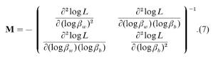
　　该方法计算速度快，因为它提供了一个估计的协方差矩阵，它显然使log和 log※。

　　This method is computationally fast and, since it provides an estimate of the covariance matrix, it obviously enables construction of confidence areas for logand log.※

　　※注：如果只估计了一个传输参数，这种似然方差方法实际上与响应变量C的广义线性模型相同，二项分布的指数S，一个互补的对数-对数链接函数，以及log(I/N)作为偏移量。因为在这种情况下，我们想同时估计两个传播参数，是不可能使用这个GLM。

　　※Note that, if only one transmission parameter is estimated, this likelihood variance method is in fact the same as a generalized linear model with response variate C, binomially distributed with index S, and a complementary log-log LINK function, and log(I/N) as offset. Because in this case we want to estimate two transmission parameters simultaneously, it is not possible to use this GLM.

　　恢复/死亡率参数使用广义线性模型估计了审查生存分析（Aitken 等人[13]）。在这个模型中，每个动物可以观察到两个解释变量Tk 和yk。第一个变量，Tk是观察到的传染期长度。第二个变量yk是一个审查变量，如果Tk是真实存活时间，yk是1，而如果真实存活时间大于Tk, yk是0。似然函数如下:

　　The recovery/death rate parameter has been estimated using a generalized linear model for survival analysis with censoring, as described by Aitken et al. [13]. In this model for each animal two explanatory variables Tk and yk can be observed. The first one, Tk  is the observed length of the infectious period. The second one, yk, is a censoring variable: yk is 1 if Tk is the true survival time, whereas yk is 0 if the true survival time is greater than Tk. The likelihood function reads as follows:

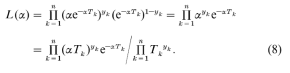
　　这个可能性的核心是一样的，是一组n观察值yk各有一个独立的泊松分布与平均值 (见[13])。用Genstat进行分析[14],使用RSURVIVAL程序，即yk表示响应变量，log为偏移量，模型配备了一个对数连接功能和泊松分布。结果是一个估计的对数和它的估计方差的估值。 以下运算给出log的估计：

　　The kernel of this likelihood is the same as it would be with a set of n observations yk each having an independent Poisson distribution with mean (see [13]). The analysis was performed in Genstat  [14], using the RSURVIVAL procedure, where yk denotes the response variate, loghe offset, and the model is fitted with a log LINK function and a Poisson distribution. The output is an estimate of log and its estimated variance. The estimator of log is given by:

　　log = log- log.                       (9)

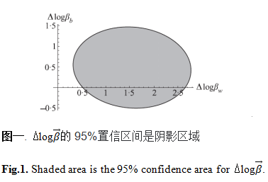
　　推导log的置信区间是通过添加log 和 log协方差矩阵得到的：

　　Derivation of a confidence area for log is done by adding the covariance matrices for log and log:

　　估计断奶猪和育肥猪的logs和var(log)s被用来构造一个置信区间差异的两个logs,并评估是否Row 和R’ob使断奶猪和育肥猪之间有明显的差异。

　　The estimated logs and var(log)s for weaner and slaughter pigs were used to construct a confidence area for the difference of the two logs, and to assess whether Row or R’ob  differ significantly between weaner and slaughter pigs.

　　未完待续

　　To be continued…